“Descriptions should be generative. A modest collection of primitives should allow description of a vast set of objects. ”
Thomas Binford [1]
One of the best ways to know that you understand a subject is when you are able to summarize it in a concise manner. Similarly, one of the recurring themes in scientific research is to explain a phenomena using simple patterns. These simple patterns allows us to interpret, predict and manipulate the world around us much more easily than if we chose more complex representations.
For example, many approaches for pose estimation and pose manipulation start by representing a person using a stick figure instead of modelling the entire human body.
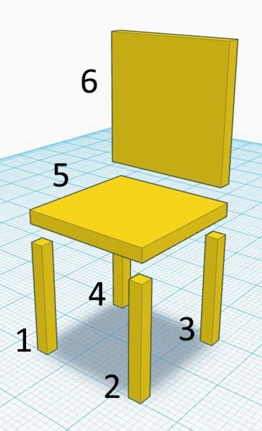
In 3D scenes the simplest representation of objects is as an assembly of basic building blocks or “primitives”. For example, we can describe a chair simply as a collection of elongated boxes – one horizontally elongated box on top of four other vertically elongated boxes and another box for the backrest.
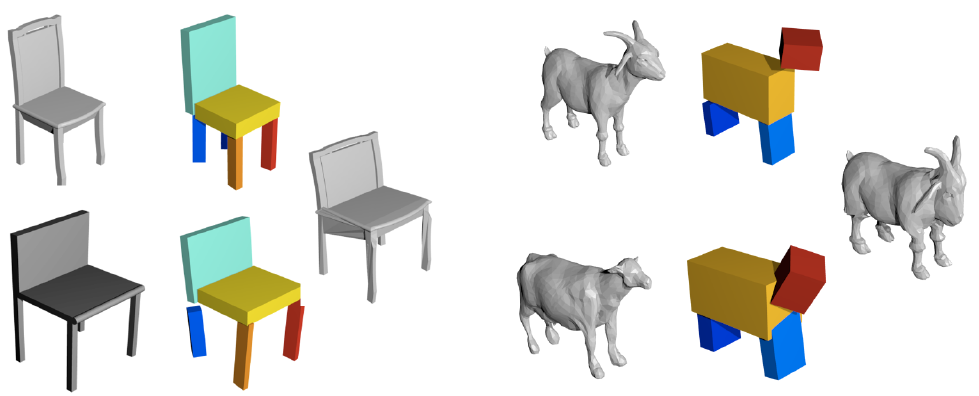
In “Learning Shape Abstraction by Assembling Volumetric Primitives” [2], Tulsiani et al. tackle the problem of approximating a 3D object in a complex representation such as a mesh representation using a simpler primitive-based representation. Specifically they suggest a method by which the object is represented using up to $M$ rectangular cuboids.

The cuboid
A rectangular cuboid is a 3D rectangle with a width, height and depth of $z=(w, h, d)$ with two additional parameters to control for its rotation and translation in space, $q, t$. Tulsiani et al. denote a cuboid in the canonical frame as untransformed and with the notation $P$ while the transformed cuboid is denoted with $\bar{P} = (z, q, t)$
Assembling the cuboids
To approximate a given shape using $M$ cuboids we start by discretizing the mesh and passing it to a 3D fully-connected convolutional network which outputs the parameters for $M$ cuboids.
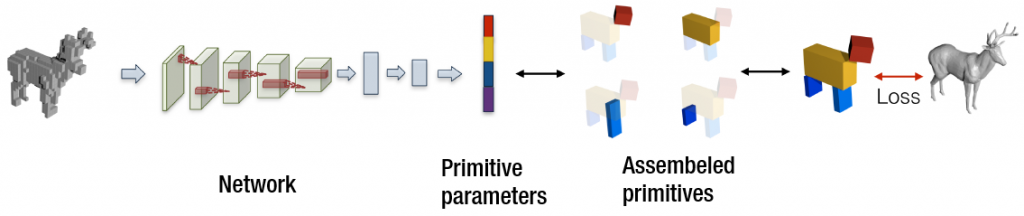
Loss function
To maintain fidelity the predicted shape is compared to the target shape and not to the discretized input, but how can we compare objects in different 3D representations in a manner that is efficient and differential?
We start by being agnostic of the 3D representations completely. To do so we use a function which calculates a distance between an object and a single point called Distance Field. For a 3D object $O$ and a point $p$ the distance field is defined as $$\mathcal{C}(p;O)=\min\limits_{p’ \in S(O)} \Vert p – p’ \Vert _2$$ where $S(\cdot)$ is the surface function. Note that $C(\cdot; O)$ evaluates to $0$ within the object interior.
We use the distance field function to define two complementary loss terms which together encourage the convergence of the predicted shape onto the target shape.
Coverage loss: $O \subseteq \cup _m \bar{P}_m$
This loss is designed to penalize the model if the target shape is not completely covered by the predicted shape. We can formalize this concept by requiring that the distance field of the assembled shape is zero with respect to points sampled on the target shape: $$L_1(\cup _m \bar{P}_m, O) = \mathbb{E}_{p \sim S(O)} \Vert \mathcal{C}(p;\cup _m \bar{P}_m) \Vert ^ 2$$
Note that $\mathcal{C}(p;\cup_m \bar{P}_m)=\min\limits_m\mathcal{C}(c;\bar{P}_m)$ which allows us to conveniently work on each primitive separately.
Calculating the distance field of cuboids
For a canonical cuboid $P$ the distance field can be computed using Pythagoras’ theorem as: $$\mathcal{C}(p; P)^2= (\vert p_x \vert – w)^2_+ + (\vert p_y \vert – h)^2_+ + (\vert p_z \vert – d)^2_+$$ we can now introduce back the translation and rotation by applying their inverse to the point $p$ instead of to the cuboid: $$ p’ = \mathcal{R}(\mathcal{T}(p, -t), \bar{q}); \; \; \mathcal{C} (p;\bar{P})= \mathcal{C}(p’, P)$$
Consistency loss: $ \cup _m \bar{P}_m \subseteq O $
This loss complements the coverage loss by encouraging the target shape to cover the predicted shape. Together with the coverage loss it tries to make the overlap between the shapes as tight as possible: $$L_2(\cup _m \bar{P}_m, O) = \sum\limits_m \mathbb{E}_{p \sim S(\bar{P}_m)} \Vert \mathcal{C}(p; O)\Vert ^ 2 $$
A few notes on sampling points
Firstly, instead of sampling from the transformed primitive $\bar{P}$ we can more easily sample from the canonical primitive $P$ and transformed the sampled points: $$p \sim S(P); \; \; p’ \sim S(\bar{P}) \equiv \mathcal{T}(\mathcal{R}(p, q), t);$$
Next, notice how the derivation of the consistency loss function for updating the model is with respect to the points sampled from the surface of the primitives. To make sure we sample from the cuboid in a uniform manner we will want to sample from each face of the cuboid in proportion to the face’s size. Unfortunately it is not straight-forward to do so in a manner that retains our ability to differentiate the loss in respect to the shape parameters. Instead we can sample equally from all faces and re-wight their contribution to the loss computation based on the proportions of the face: $$L_2(\cup _m \bar{P}_m, O) = \sum_m \sum_{p, w_p \sim S(\bar{P}_m)} w_p \Vert \mathcal{C}(p;O) \Vert ^2$$
A final point worth making here is that we need to use the re-parameterization trick when sampling the actual points. Assume we sample from cuboid $P$ from the face were $x=w$. We can sample from two uniform variables: $$u_x = 1; u_y \sim [-1, 1]; u_z \sim [-1, 1]$$ Then we can define the sampled point as: $$p = (u_x w, u_y h, u_z d))$$ By defining such a process for all faces we can easily calculate the derivaties w.r.t. the primitive itself.
In general, whenever you see a place where you need to sample or select something, there is a good chance that you cannot directly differentiate your action. Take for example sampling a point from a face of a cuboid. Instead of sampling uniformly $p_w \sim [-w, w]$ we sample $u_w \sim [-1, 1]$ and then set $p’_w = u_w \cdot w$, but why? the first option is much less complicated!
The answer is that there is no clear way to calculate the derivatives of the result of the action (whatever $p_w$ is taking part of) and the parameters we wish to learn ($w$). What exactly is $\dfrac{\partial{p’_w}}{\partial(w)}$? In other words – how would the value sampled from $[-w, w]$ change if we slightly changed $w$? This is obviously a very tough question and in may cases impossible to answer.
By using the re-parameterization trick we take the actual sampling out of the equation – the way $p’_m$ changes w.r.t. $w$ is very easy to calculate.
A natural question at this point would be – why didn’t we need the re-parameterization trick earlier, when we sampled points for the coverage loss? Because those points were sampled from the target shape and thus the sampling did not appear in the derivation chain w.r.t. the model parameters.
Variable number of primitives
So far we have assumes that the number of primitives is always $M$, but the number of cuboids needed to describe a chair is not necessarily the same needed for a giraffe. You could even have different chairs described with a different number of cuboids (e.g. with or without a backrest). If we allow the network to output a variable amount of primitives we allow it to adapt the complexity of the predicted shape as needed.
We achieve this by assigning to every primitive $P_i$ a variable sampled from the Bernoulli distribution: $z^e_i \sim Bern(P_i)$. When $z^e_i = 0$ we simply ignore the cuboid $P_i$ when assembling the predicted shape. This means that our predicted shape can be comprised of any number of primitives up to $M$. To sample the variable we simply add it to the primitive representation predicted by the network.
Effect on loss function
How does not having a primitive affect the loss functions?
For calculating the consistency loss we can simply ignore it when sampling points on the predicted shape.
When considering the coverage loss we remember that $\mathcal{C}(p;\cup_m \bar{P}_m)=\min\limits_m\mathcal{C}(c;\bar{P}_m)$ and therefore by replacing $ \mathcal{C}(c;\bar{P}_i)$ with a $\infty$ would make sure that $P_i$ does not affect the loss.
In order to learn the actual parameter $z^e_i$ we use the REINFORCE algorithm which allows us to train the network with respect to an arbitrary feedback signal, using a signal corresponding to an overall low loss function as well as a parsimony reward to encourage using fewer primitives.
Results
Tulsiani et al. covered several applications for this method in the paper which essentially build on the shape embedding that the network creates and its inherent structure to find interesting interactions they can use it for.
One of the uses that they showed in the paper that I found very interesting is projecting one object onto another.
This is done by assigning points from the mesh of object $A$ to a location on the nearest primitive in its predicted shape $A’$ and then transforming those points based on the transformation between $A’$ and the predicted shape of the target object, $B’$.
This method gives us a lot of power to manipulate the given objects as it is far easier to describe manipulations of simple primitive shapes than of complex meshes.
Conclusions
First, a disclaimer: Although this is the first paper that I have read that deals with this problem, it is not new (CVPR 2017) and I would expect that in most ways it has already been surpassed and that the points I would make below were already answered in other papers. Hopefully I would get to them soon.
This paper surprised me. Going in I expected it to use some sort of sequential model to generate the primitives but in its simplicity it actually achieved something that a sequential model would be hard to replicate – by having a single output vector it allows the network to define “roles” for every primitive in a certain class, e.g. primitive $i$ is a chair’s backrest and $i+1$ is the seat, and this opens up very powerful ways to compare and manipulate class objects.
While this trait might arise naturally in a sequential model if it, for example, learns to cover the space in a specific pattern, I would expect it to be non-trivial to engineer. Instead I would probably attach an identifier to every primitive and add a loss term which constrains the relationship between the primitives based on the identifier.
A more “unsupervised” approach would be to simply cluster the primitives based on their properties (either cuboid parameter or primitive embeddings).
Finally, as someone who came from the world of 2D images it seems rather limited that they train a different model for every category (chair, plane, animal). This is especially conspicuous as they stress that their method is “data-driven”, and I would have expected that increasing and diversifying the data would have more benefits than challenges. I hope future papers do tackle this issue.
All in all it was a very interesting and well-written paper with very intriguing results. I certainly look forward to the next paper in this topic.
- [1]T. O. Binford and J. M. Tenenbaum, “Computer vision,” Computer, pp. 19–24, May 1973, doi: 10.1109/mc.1973.6536714.