I have been trying to wrap my head around the way PixelCNN++ is using discretized mixture of logistic distributions to sample pixels and could not find a single comprehensive source about it, so in the following post I would try to combine (and refine) all of the sources I could find (Specifically, the most comprehensive source I found is a github comment by Rayhane-mama and this post draws heavily on it).

So first of, what are we trying to do and why? In the original PixelCNN architecture each channel in a pixel is modelled as a distribution using a 255-way softmax layer, which is basically a 255-way classification model. But pixel values are not categorical and the difference between a value of 255 and 128 should be more pronounced than between 255 and 254, but instead of incorporating this information into our modelling we waste precious training resources while the model learns this fact.

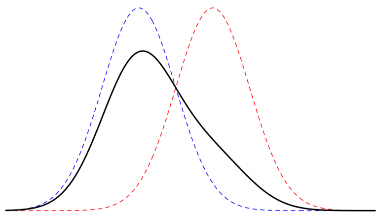
A different tack is to learn a continuous distribution over the pixel values and then discretize it into 255 bins, which is what was proposed in PixelCNN++. Instead, the distribution of pixel values is modelled as a mixture of logits which is then discretized: $$\upsilon \sim \sum_{i=1}^K \pi_i \cdot \mathrm{logistic}(\mu_i, s_i)$$ Here $\pi_i$ is the weight given for a logistic distribution $i$ with parameters $\mu_i, s_i$.

Now that we defined our distribution we want to be able to do 3 things: train a model w.r.t. the distribution, sample from the distribution and discretize the distribution.

Distcretizing the distribution

Lets start from the end. Assuming we have learned a mixture as defined above, how can we estimate the probability of a given pixel? We have defined the probability in terms of continuous distributions so the first thing we need to do is bin the pixel values back to discrete values. This means that the probability of getting a specific value $x$ is the sum of the probabilities for $x \pm 0.5$: $$P(round(\upsilon)=x) = P(x – 0.5 \leq \upsilon \leq x + 0.5) = P(\upsilon \leq x + 0.5) – P(\upsilon \leq x – 0.5) = F_\upsilon(x + 0.5) – F_\upsilon(x – 0.5)$$ Where $F_\upsilon$ is the CDF of $\upsilon$. Subbing the above into our previous definition with respect to the CDF of a logistic distribution we get: $$P(x | \pi, \mu, s) = \sum_{i=1}^K \pi_i \cdot \left[ \sigma \left( \dfrac{x+0.5 – \mu_i}{s_i} \right) – \sigma \left( \dfrac{x -0.5 – \mu_i}{s_i} \right) \right]$$

Sampling

Sampling consists of two steps – sampling the logistic distribution from the mixture and sampling a value from that distribution.

It can be difficult to sample from an arbitrary distribution, and I highly recommend going over these slides to understand the general picture better. Fortunately for us the CDF of a logistic distribution is invertible which means we can use a very simple approach. Given a probability $p$, the inverse CDF (Quantile function) gives us a value $x$ such that the probability of getting a value $x$ or lower from our distribution is $p$. We use this fact by sampling a probability from the uniform distribution $u \sim U(0,1)$ and taking the value we get from the inverse CDF function. Specifically for the logistic distribution the function we use is: $$x_i = \mu_i + s_i \cdot log \left( \dfrac{u}{1-u} \right)$$

To select the actual distribution we sample from we can simply take $argmax_i{\pi_i}$, but in practice this leads to a lower quality of results.
Instead we will use the Gumbel-softmax trick. In essence we add randomness by adding the logits of the mixture probabilities with random values sampled from the gumbel distribution: $$g_i \sim -log(-log(Uniform(0,1))$$ To do the actual selection we will use the softmax-with-temperature: $$y_i = \dfrac{e^{(log(\pi_i + g_i)/\tau}}{\sum_{j=1}^K e^{(log(\pi_j + g_j)/\tau} }$$ This converges to the discrete argmax operation with $\tau \to 0_+$ while maintaining the order between the mixture weights as well as being differentiable w.r.t. them.

Training

Lets start with training a single logistic distribution. We have some model which outputs the distribution parameters $\pi_i, \mu_i, log{s_i}$ and we have a real sample point $x$. How can we use gradient descent to improve our maximum likelihood? As we’ve seen when discretizing the distribution, the probability at point $x$ isn’t just for that point, instead it incorporates the probability for the entire bin of $x \pm 0.5$ and we can increase this by maximizing the CDF delta between those two points: $$ \sigma \left( \dfrac{x+0.5 – \mu_i}{s_i} \right) – \sigma \left( \dfrac{x -0.5 – \mu_i}{s_i} \right) $$ Another way to visualize this process is by remembering that the CDF is the integral of the PDF and by maximizing the difference in the neighborhood around $x$ we are also maximizing the derivative at that point, i.e. maximizing the increase in PDF.

Corner cases

The above fails when $x=0$ or $x=1$ as we overflow on either side ($\pm 0.5$). Instead we replace that value with $Sigmoid \left( \dfrac{\infty – \mu_i}{s_i} \right)$ when $x=1$ and $Sigmoid \left( \dfrac{-\infty – \mu_i}{s_i} \right)$ when $x=0$ .

In summary, we calculate the PDF in point $x$ by to calculating the difference between of $x + 0.5$ and $x – 0.5$ for the function: $$\Delta CDF(x) = \begin{cases} Sigmoid \left( \dfrac{\infty – \mu_i}{s_i} \right) , \quad x=1 \\ Sigmoid \left( \dfrac{-\infty – \mu_i}{s_i} \right) , \quad x=0 \\ Sigmoid \left( \dfrac{x + 0.5- \mu_i }{s_i} \right) – Sigmoid \left( \dfrac{x – \0.5- \mu_i }{s_i} \right) , \quad o.w \end{cases} $$

Selecting from the mixture

The vector $\pi$ represents the weights over the different distributions. By using a Softmax on top of it we make sure that it is a proper distribution. Denoting $X$ as the vector of CDF deltas we got in the previous step, we can use this new distribution to encourage the selection of the best logistic distribution: $X \cdot Softmax(\pi)$. Finally, for numeric stability we actually do: $$LogSumExp \left(log(X) + log(\pi) \right)$$